E Supp. materials for ch. 4
E.1 Confidence button presses
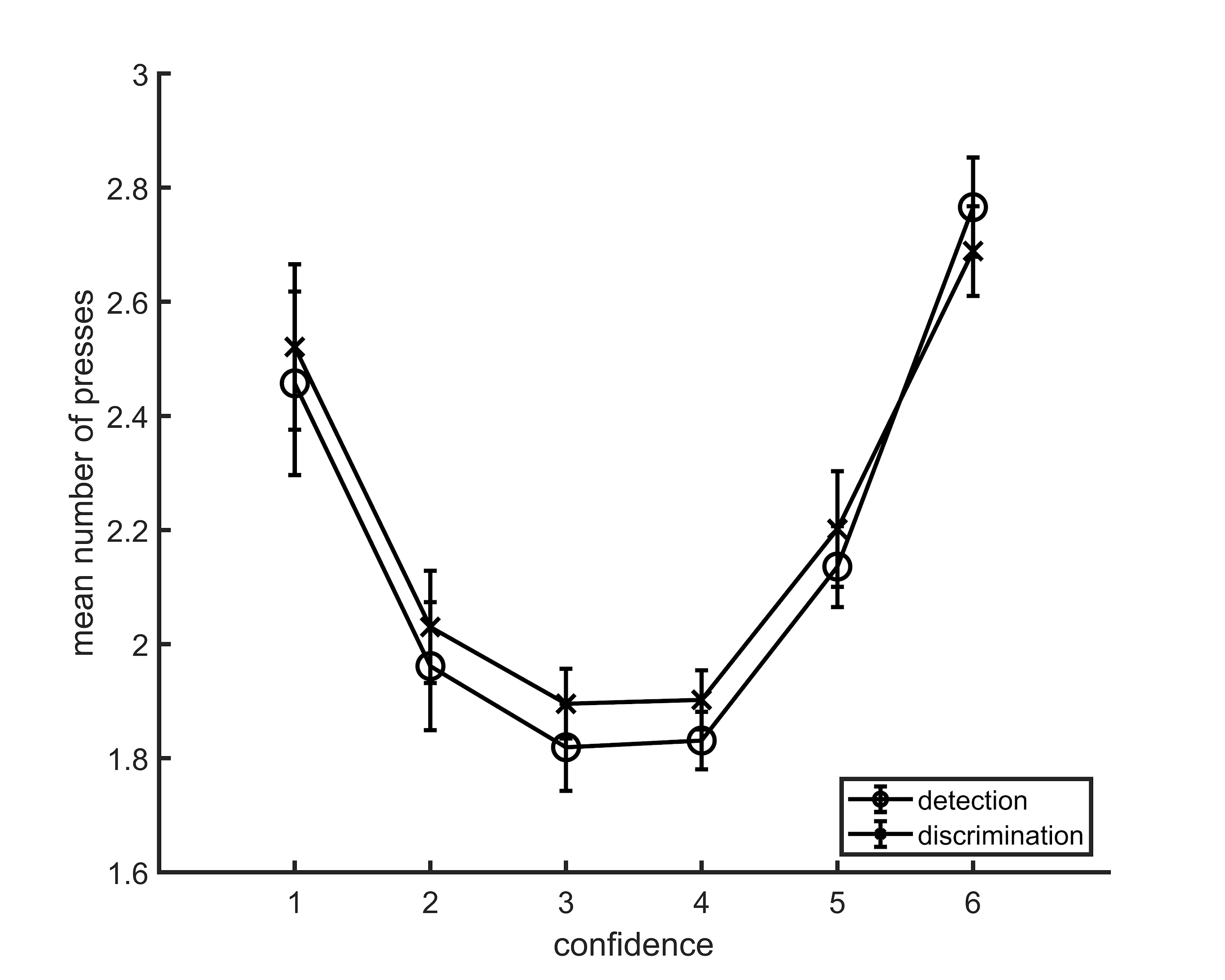
Figure E.1: Average number of button presses for each confidence level, as a function of task. More button presses were needed on average to reach the extreme confidence ratings, hence the quadratic shape. No difference between the two tasks was observed in the mean number of button presses for any of the confidence levels. Error bars represent the standard error of the mean.
E.2 zROC curves
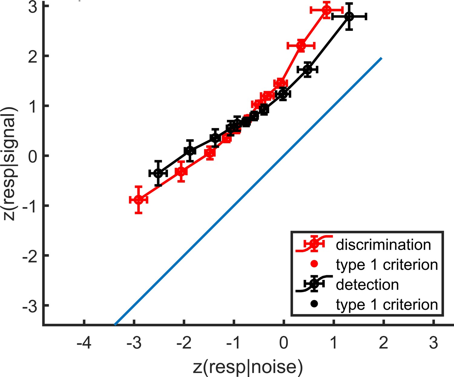
Figure E.2: mean zROC curves for the discrimination and detection tasks. As expected in a uv-SDT setting, the discrimination curve is approximately linear with a slope of 1, and the detection curve is approximately linear with a shallower slope. Error bars represent the standard error of the mean.
E.3 Global confidence design matrix
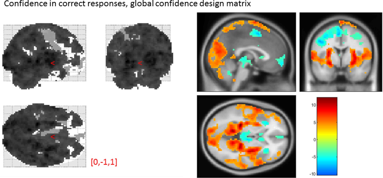
Figure E.3: Effect of confidence in correct responses, from the global-confidence design matrix. Uncorrected, thresholded at p<0.001. Left: glass brain visualization of the whole brain contrast. Right: yellow-red represent a positive correlation with subjective confidence ratings, and green-blue represent a negative correlation.
From our pre-specified ROIs, only the vmPFC and BA46 ROIs showed a significant linear effect of confidence in correct responses, in the opposite direction to what we expected based on previous studies. This is likely to be due to the differences in confidence profiles between the detection and discrimination tasks:
| Average beta | T value | P value | Standard deviation | |
|---|---|---|---|---|
| vmPFC | -0.35 | -3.06 | 4 × 10⁻³ | 0.67 |
| pMFC | -0.31 | -2.48 | 0.02 | 0.74 |
| precuneus | 0.25 | 2.30 | 0.03 | 0.64 |
| ventral striatum | -0.056 | -1.51 | 0.14 | 0.22 |
| FPl | 0.16 | 1.52 | 0.14 | 0.64 |
| FPm | -0.12 | -1.46 | 0.16 | 0.48 |
| BA 46 | 0.37 | 3.77 | 6 × 10⁻⁴ | 0.57 |
E.4 Effect of confidence in our pre-specified ROIs
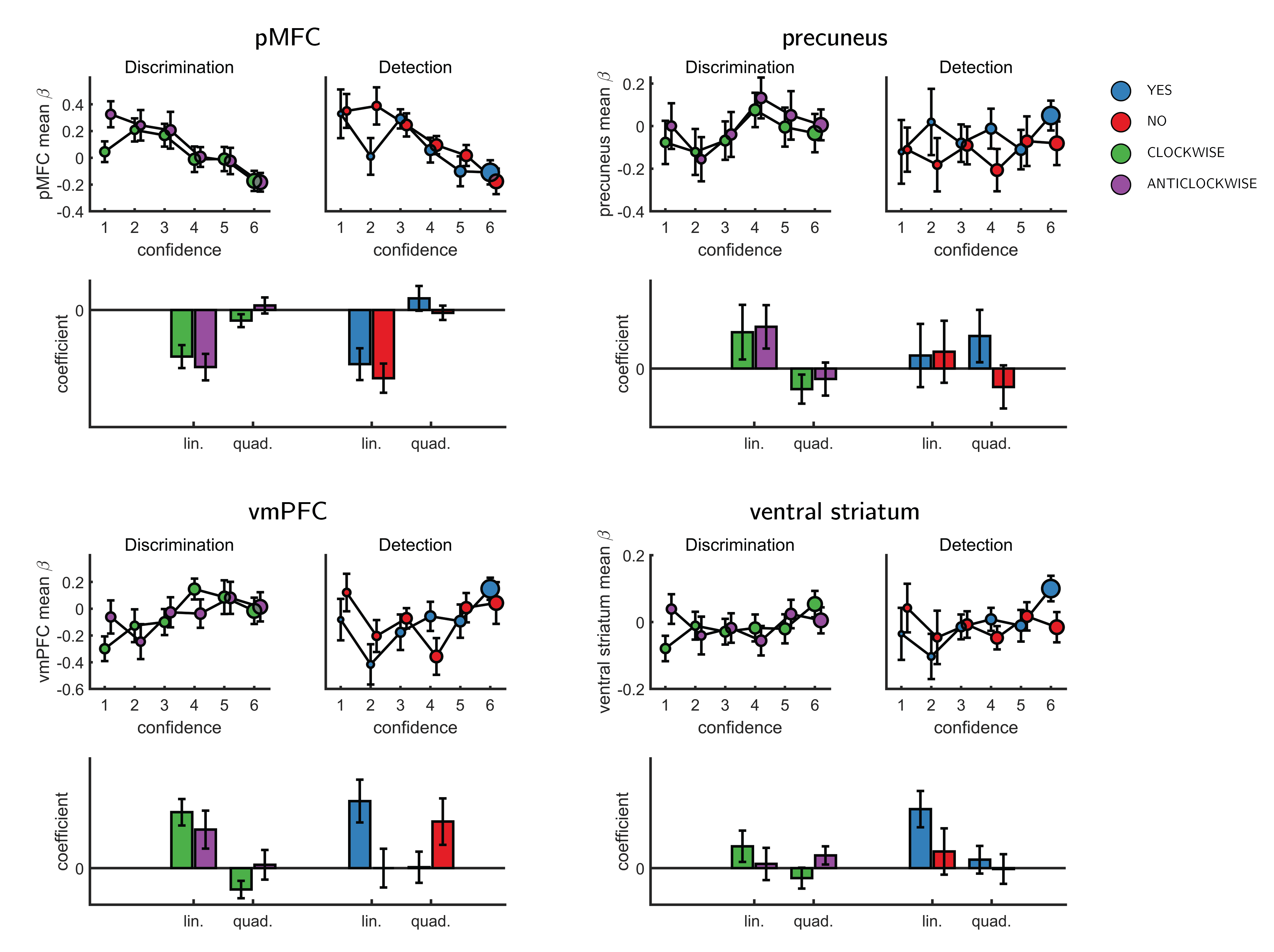
Figure E.4: Effect of confidence in all 4 ROIs, as a function of task and response, as extracted from the categorical design matrix. No significant interaction between the linear or quadratic effects and task or response was observed in any of the ROIs.
E.5 SDT variance ratio correlation with the quadratic confidence effect
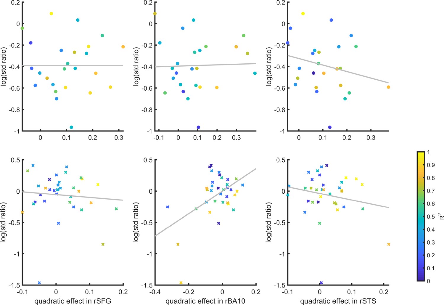
Figure E.5: Inter-subject correlation between the quadratic effect in the right hemisphere clusters and the ratio between the detection (top panel) and discrimination (lower panel) distribution variances, as estimated from the zROC curve slopes in the two tasks. Marker color indicates the goodness of fit of the second-order polynomial model to the BOLD data. All Spearman correlation coefficients are <0.25.
E.6 Correlation of metacognitive efficiency with linear and quadratic confidence effects
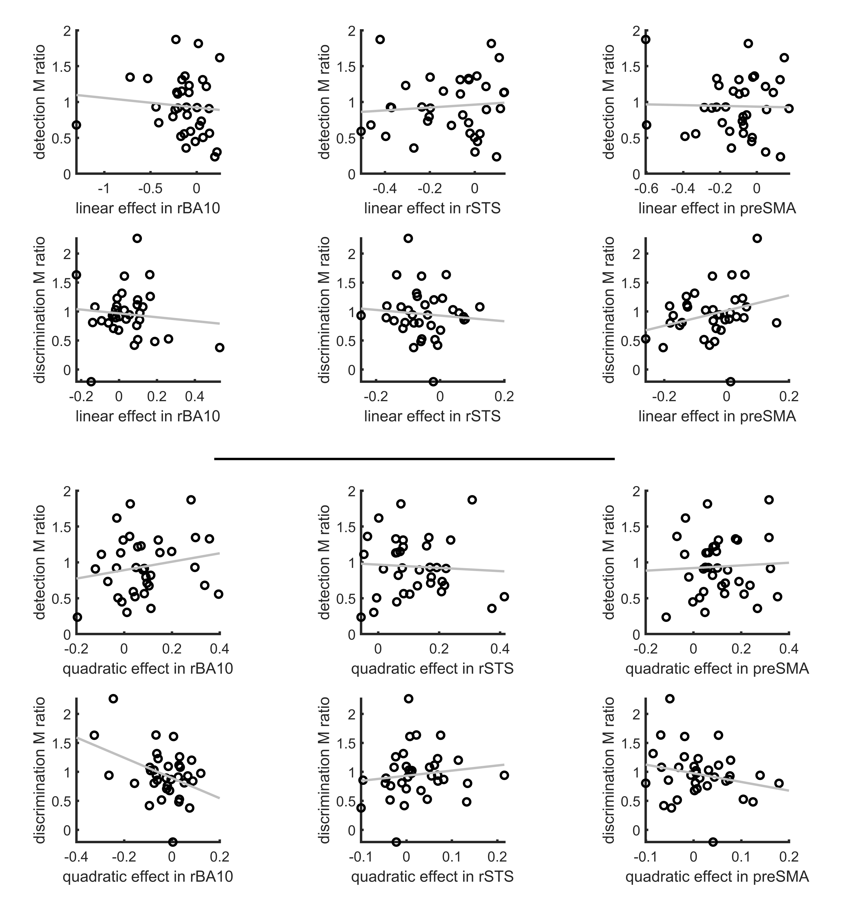
Figure E.6: Inter-subject correlation between the linear (upper panel) and quadratic (lower panel) effects in the right hemisphere clusters and metacognitive efficiency scores (measured as M ratio = meta-d’/d’, Maniscalco and Lau, 2012).
E.7 Confidence-decision cross classification
In order to dissociate between brain regions that encode stimulus visibility and brain regions that encode decision confidence, we performed a multivariate cross-classification analysis. We trained a linear classifier on detection decisions (‘yes’ and ‘no’), and tested it on discrimination confidence (high and low), and vice versa. Shared information content between detection responses and confidence in discrimination is expected in brain regions that encode stimulus visibility, rather than accuracy estimation. In detection, yes responses are associated with higher stimulus visibility compared to no responses (regardless of decision confidence), and in discrimination high confidence trials are associated with higher visibility than low confidence trials (regardless of subjective confidence).
Presented cross classification scores are the mean of cross classification accuracies in both directions. Detection-response and discrimination-confidence cross-classification was significantly above chance in in the pMFC (\(t(29)=2.76, p<0.05\), corrected for family-wise error across the four ROIs), and in the BA46 anatomical subregion of the frontopolar ROI (\(t(29)=2.64, p<0.05\), corrected).
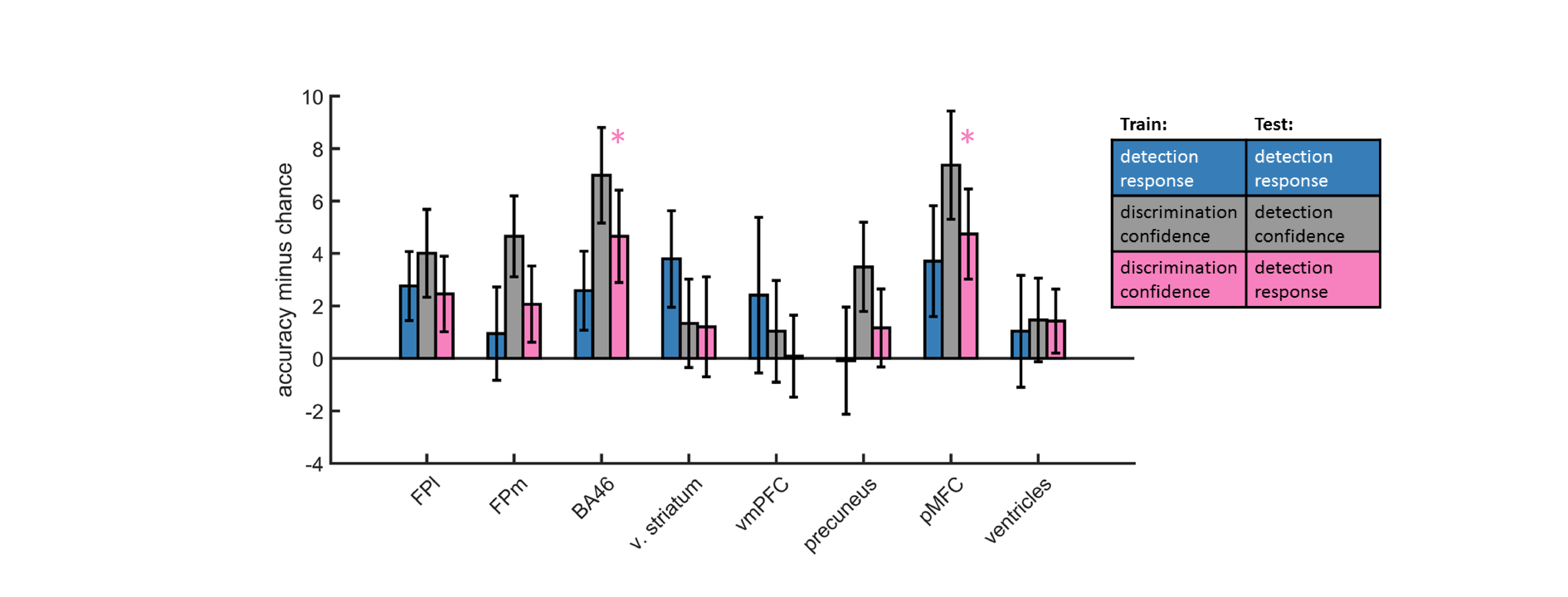
Figure E.7: Accuracy minus chance for classification of response in detection (yes vs. no; blue), and from a cross-classification between tasks: confidence in detection and confidence in discrimination (gray), and confidence in discrimination and decision in detection (pink).
E.8 Static Signal Detection Theory
E.8.1 Discrimination
Generative model
According to SDT, a decision variable \(x\) is sampled from one of two distributions on each experimental trial.
\[\begin{equation} \mu_t=\begin{cases} 0.5, & \text{if cw}.\\ -0.5, & \text{if acw}.\\ \end{cases} \end{equation}\]
\[\begin{equation} x_t \sim \mathcal{N}(\mu_t,1) \end{equation}\]
Inference
\(x\) is compared against a criterion to generate a decision about which of the two distributions was most likely, given the sample. For a discrimination task with symmetric distributions around 0, the optimal placement for a criterion is at 0.
\[\begin{equation} decision_t=\begin{cases} \text{cw}, & \text{if } x_t>0.\\ \text{acw}, & \text{else}. \end{cases} \end{equation}\]
In standard discrimination tasks, a common assumption is that the two distributions are Gaussian with equal variance. This assumption has a convenient computational consequence: the log-likelihood ratio (LLR), a quantity that reflects the degree to which the sample is more likely under one distribution or another, is linear with respect to \(x\). Confidence is then assumed to be proportional to the distance of \(x_t\) from the decision criterion.
In what follows \(\phi(x,\mu,\sigma)\) is the likelihood of observing x when sampling from a normal distribution with mean \(\mu\) and standard deviation \(\sigma\).
\[\begin{equation} LLR = log(\phi(x_t,0.5,1))-log(\phi(x_t,-0.5,1)) \end{equation}\]
\[\begin{equation} confidence_t \propto |x_t| \end{equation}\]
E.8.2 Detection
Generative model
A common assumption is that in detection the signal distribution is wider than the noise distribution [unequal-variance SDT; Wickens (2002), 48].
\[\begin{equation} \mu_t=\begin{cases} 1.3, & \text{if P}.\\ 0, & \text{if A}.\\ \end{cases} \end{equation}\]
\[\begin{equation} \sigma_t=\begin{cases} 2, & \text{if P}.\\ 1, & \text{if A}.\\ \end{cases} \end{equation}\]
\[\begin{equation} x_t \sim \mathcal{N}(\mu_t,\sigma_t) \end{equation}\]
Inference
Here \(med(x)\) represents the median sensory sample \(x\). This criterion was chosen to ensure that detection responses are balanced.
\[\begin{equation} decision=\begin{cases} \text{P}, & \text{if } x_t>med(x).\\ \text{A}, & \text{else}. \end{cases} \end{equation}\]
Importantly, in uv-SDT, LLR is quadratic in x. \[\begin{equation} LLR = log(\phi(x,1.3,2))-log(\phi(x,0,1)) \end{equation}\]
\[\begin{equation} confidence \propto |x_t-med(x)| \end{equation}\]
E.9 Dynamic Criterion
In SDT, task performance depends on the degree of overlap between the underlying distributions (d’) and on the positioning of the decision criterion (c). Participants may optimize criterion placement based on their changing beliefs about the underlying distributions (Ko & Lau, 2012). To model this dynamic process of criterion setting we simulated a model where beliefs about the underlying distributions are the Maximum Likelihood Estimates of the mean and standard deviation, based on the last 5 samples that were (correctly or not) categorized.
E.9.1 Discrimination
Generative model
As in the Static Signal Detection model.
Inference
Means and standard deviations of the two distributions are estimated based on the last 5 samples in each category. To model prior beliefs about these parameters, each participant starts the task with 5 imaginary samples from the veridical distributions. Means and standard deviations are then extracted from these imaginary samples. In what follows, \(\vec{cw}\) and \(\vec{acw}\) are vectors with entries corresponding to the last 5 samples that were (correcly or not) labelled as ‘cw’ and ‘acw,’ respectively. \(\bar{x}_{cw}\) and \(\bar{x}_{acw}\) correspond to the sample means of these vectors. \(\sigma_{cw}\) and \(\sigma_{acw}\) correspond to their standard deviations.
\[\begin{equation} LLR = log(\phi(x,\bar{x}_{cw},\sigma_{cw}))-log(\phi(x,\bar{x}_{acw},\sigma_{acw})) \end{equation}\]
Decisions and confidence are extracted from the \(LLR\) as in the Static Signal Detection model.
E.9.2 Detection
Generative model
As in the Static Signal Detection model.
Inference
As in discrimination. In what follows, \(\vec{a}\) and \(\vec{p}\) are vectors with entries corresponding to the last 5 samples that were (correcly or not) labelled as ‘signal absent’ and ‘signal present,’ respectively. \(\bar{x}_{a}\) and \(\bar{x}_{p}\) correspond to the sample means of these vectors. \(\sigma_{a}\) and \(\sigma_{p}\) correspond to their standard deviations.
\[\begin{equation} LLR = log(\phi(x,\bar{x}_{p},\sigma_{p}))-log(\phi(x,\bar{x}_{a},\sigma_{a})) \end{equation}\]
In detection, \(LLR=0\) at two points (see figure @ref{fig:models). The decision criterion \(c_t\) is chosen to coincide with the rightmost point, which is positioned between the Signal and Noise distribution means.
\[\begin{equation} decision=\begin{cases} \text{p}, & \text{if } x_t>c_t.\\ \text{a}, & \text{else}. \end{cases} \end{equation}\]
\[\begin{equation} confidence \propto |LLR| \end{equation}\]
E.10 Attention Monitoring
Similar to the Dynamic Criterion model, in the Attention Monitoring model participants adjusts a decision criterion based on changing beliefs about the underlying distributions. However, unlike the Dynamic Criterion model, here beliefs change not as a function of recent perceptual samples, but as a function of access to an internal variable that represents the expected sensory precision (attention).
E.10.1 Discrimination
Generative model
In our schematic formulation of this model, participants have a true attentional state, which for simplicity we treat as either being on (1) or off (0). When attending, participatns enjoy higher sensitivity than when they don’t.
\[\begin{equation} p(attended_t)= 0.5 \end{equation}\]
The attentional state determines the means of sensory distributions.
\[\begin{equation} \mu_t=\begin{cases} 0.5, & \text{if cw and $\neg attended_t$}.\\ -0.5, & \text{if acw and $\neg attended_t$}.\\ 2, & \text{if cw and $attended_t$}.\\ -2, & \text{if acw and $attended_t$}.\\ \end{cases} \end{equation}\]
\[\begin{equation} x_t \sim \mathcal{N}(\mu_t,1) \end{equation}\]
However, they don’t have direct access to their attentional state, but only to a noisy approximation of the probability that they were attending.
\[\begin{equation} onTask_t \sim \begin{cases} Beta(2, 1), & \text{if $attended_t$}.\\ Beta(1, 2), & \text{if $\neg attended_t$}.\\ \end{cases} \end{equation}\]Inference
Participants are then assumed to use their knowledge about the \(onTask\) variable when making a decision and confidence estimate.
\[\begin{equation} \begin{aligned} p(x_t | \text{cw}) = p(attended_t | onTask_t) \phi(x_t,2,1) + p(\neg attended_t | onTask_t) \phi(x_t,0.5,1)\\ = onTask_t \phi(x_t,2,1) + (1-onTask_t) \phi(x_t,0.5,1) \end{aligned} \end{equation}\]
\[\begin{equation} \begin{aligned} p(x_t | \text{acw}) = p(attended_T | onTask_t) \phi(x_t,-2,1) + p(\neg attended_t | onTask_t) \phi(x_t,-0.5,1)\\ = onTask_t \phi(x_t,-2,1) + (1-onTask_t) \phi(x_t,-0.5,1) \end{aligned} \end{equation}\]
\[\begin{equation} LLR = log(p(x_t | \text{w}))-log(p(x_t | \text{acw}) \end{equation}\]
\[\begin{equation} decision_t=\begin{cases} \text{cw}, & \text{if } LLR>0.\\ \text{acw}, & \text{else}. \end{cases} \end{equation}\]
\[\begin{equation} confidence_t \propto |LLR| \end{equation}\]
E.10.2 Detection
Generative model
In detection, attentional states only affect the signal distribution, as noise is always centred at 0.
\[\begin{equation} \mu_t=\begin{cases} 0, & \text{if a and $\neg attended_t$}.\\ 0.5, & \text{if p and $\neg attended_t$}.\\ 0, & \text{if a and $attended_t$}.\\ 2, & \text{if p and $attended_t$}.\\ \end{cases} \end{equation}\]
\[\begin{equation} x_t \sim \mathcal{N}(\mu_t,1) \end{equation}\]
Inference
\[\begin{equation} \begin{aligned} p(x_t | \text{p}) = p(attended_t | onTask_t) \phi(x_t,2,1) + p(\neg attended_t|onTask_t) \phi(x_t,0.5,1)\\ = onTask_t \phi(x_t,2,1) + (1-onTask_t) \phi(x_t,0.5,1) \end{aligned} \end{equation}\]
The likelihood of observing \(x_t\) if no stimulus was presented is independent of the attention state.
\[\begin{equation} \begin{aligned} p(x_t | \text{a}) = p(attended_t | onTask_t) \phi(x_t,0,1)) + p(\neg attended_t | onTask_t) \phi(x_t,0,1)\\ = \phi(x_t,0,1) \end{aligned} \end{equation}\]
\[\begin{equation} LLR = log(p(x_t | \text{p}))-log(p(x_t | \text{a}) \end{equation}\]
\[\begin{equation} decision_t=\begin{cases} \text{p}, & \text{if } LLR>0.\\ \text{a}, & \text{else}. \end{cases} \end{equation}\]
Nevertheless, confidence in judgments about stimulus absence is dependent on beliefs about the attentional state. This is mediated by the effect of attention on the likelihood of observing \(x_t\) if a stimulus were present. This is the counterfactual part.
\[\begin{equation} confidence_t \propto |LLR| \end{equation}\]