A Signal Detection Theory
“Signal Detection Theory” is a conceptual framework for the description of decision making between two alternatives in the presence of uncertainty. Examples include deciding whether a presented word has been studied before or not, to which of two groups does a noisy stimulus belong, or whether a stimulus was presented on the screen or not (Stanislaw & Todorov, 1999; Tanner Jr & Swets, 1954). Under this framework, on each experimental trial a “decision variable” is sampled from one of two distributions. I will refer to these distributions here as the signal and noise distributions, although depending on context they can have different labels, such as old and new distributions in recognition memory task or right and left in a movement discrimination task. On trials in which the decision variable exceeds a criterion \(c\), a ‘yes’ response is executed, otherwise a ‘no’ response is executed (see Fig. A.1).
(ref:app1-SDT-caption) Distribution of the decision variable across noise and signal trials, showing d’, c, and the likelihoods. Figure based on Stanislaw & Todorov, 1999.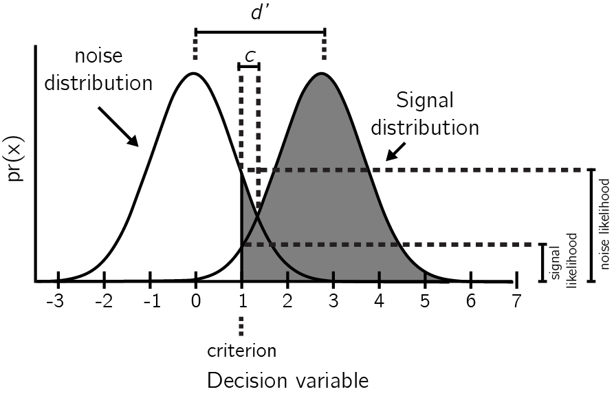
Figure A.1: (ref:app1-SDT-caption)
Given the noisiness of the incoming input, some signal trials will result in a ‘no’ response and some noise trials will result in a ‘yes’ response. This makes a total of four groups of trials that can be ordered in a two by two table:
| response | signal | noise |
|---|---|---|
| ‘yes’ | hit | false alarm |
| ‘no’ | miss | correct rejection |
Two conditional probabilities are sufficient to provide a full description of the behaviour profile of a participant, namely \(p(yes|Signal)\) (the ‘hit rate’), and \(p(yes|Noise)\) (the ‘false alarm rate’). SDT makes it possible to translate these two probabilities to properties of the signal and noise distributions and their positioning with respect to the decision criterion. The parameter \(d'\) represents the distance between the two distributions in standard deviations. Under the assumption of equal variance of the two distributions \(d'\) can be approximated as \(\hat{d'}=Z(h)-Z(f)\), with \(Z\) representing the inverse cumulative normal distribution. The parameter \(\lambda\) stands for the position of the criterion relative to the mean of the noise distribution, and can be approximated as \(\hat{\lambda}=-Z(f)\).
A.1 ROC and zROC curves
The false alarm and hit rates are often insufficient to provide a full description of a system. For example, they are not sufficient to determine the ratio between the variance terms of the two distributions, and therefore to decide if the equal variance assumption holds. To obtain a fuller picture, false alarm and hit rates can be recorded under different settings of the decision criterion. One way to experimentally shift the criterion is by manipulation of the task incentive structure. For example, in order to encourage participants to make more ‘no’ responses, rewards for correct rejections can be set higher than rewards for hits. Alternatively, confidence ratings can be collected for every decision. The criterion can then be theoretically placed between every two possible confidence ratings, to generate a full set of false positive and hit rates.
A “Receiver Operating Characteristic” (ROC) curve is the plot of false alarm and hit rates for all possible settings of a decision criterion value. It can be approximated by plotting the false alarm and hit rates for the criterion values available by the experimental manipulation (see figure ). For a system that performs at chance, false positive and hit rates should be equal for every criterion, giving rise to an ROC that follows the identity line. The area under the ROC curve (“AUROC”) can be interpreted as the proportion of times the system will identify the stimulus in a 2AFC task where noise and signal are presented simultaneously (Stanislaw & Todorov, 1999).
(ref:app1ROCcaption) Receiver Operating Characteristic (ROC) curve. Three points on the ROC curve are shown (open squares). The area under the curve, as estimated by linear extrapolation, is indicating by hatching; the true area includes the gray regions. Figure based on Stanislaw & Todorov, 1999.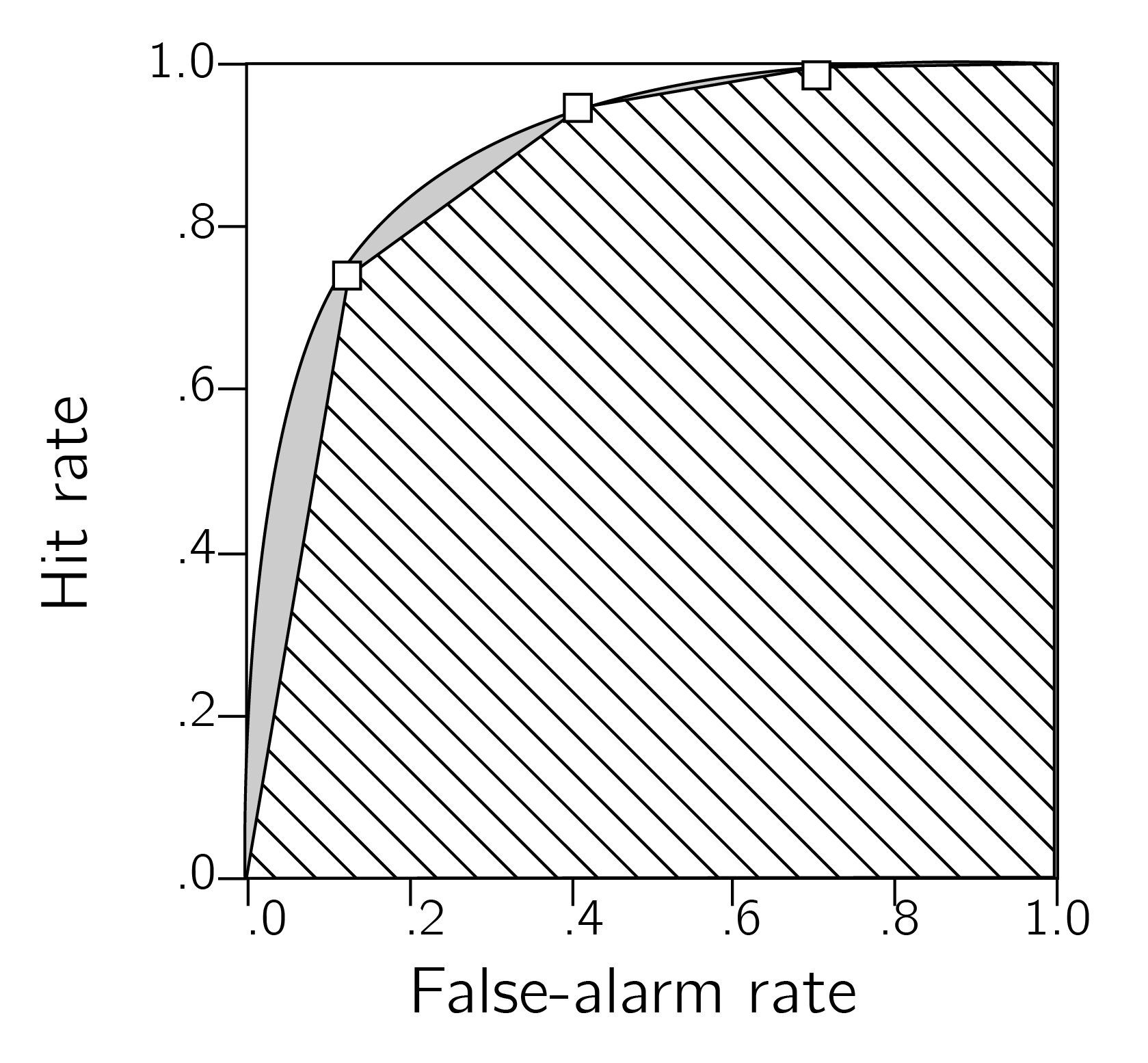
Figure A.2: (ref:app1ROCcaption)
Often it is informative to plot the inverse of the cumulative distribution for \(p(f)\) and \(p(h)\), resulting in what is known as a “zROC curve” (see figure ). The zROC curve is linear when the noise and signal distributions are approximately normal. The slope of the zROC curve equals the ratio between the standard deviations of the noise and signal distributions (Stanislaw & Todorov, 1999). Hence, the standard equal-variance SDT model predicts a linear zROC curve with a slope of 1.
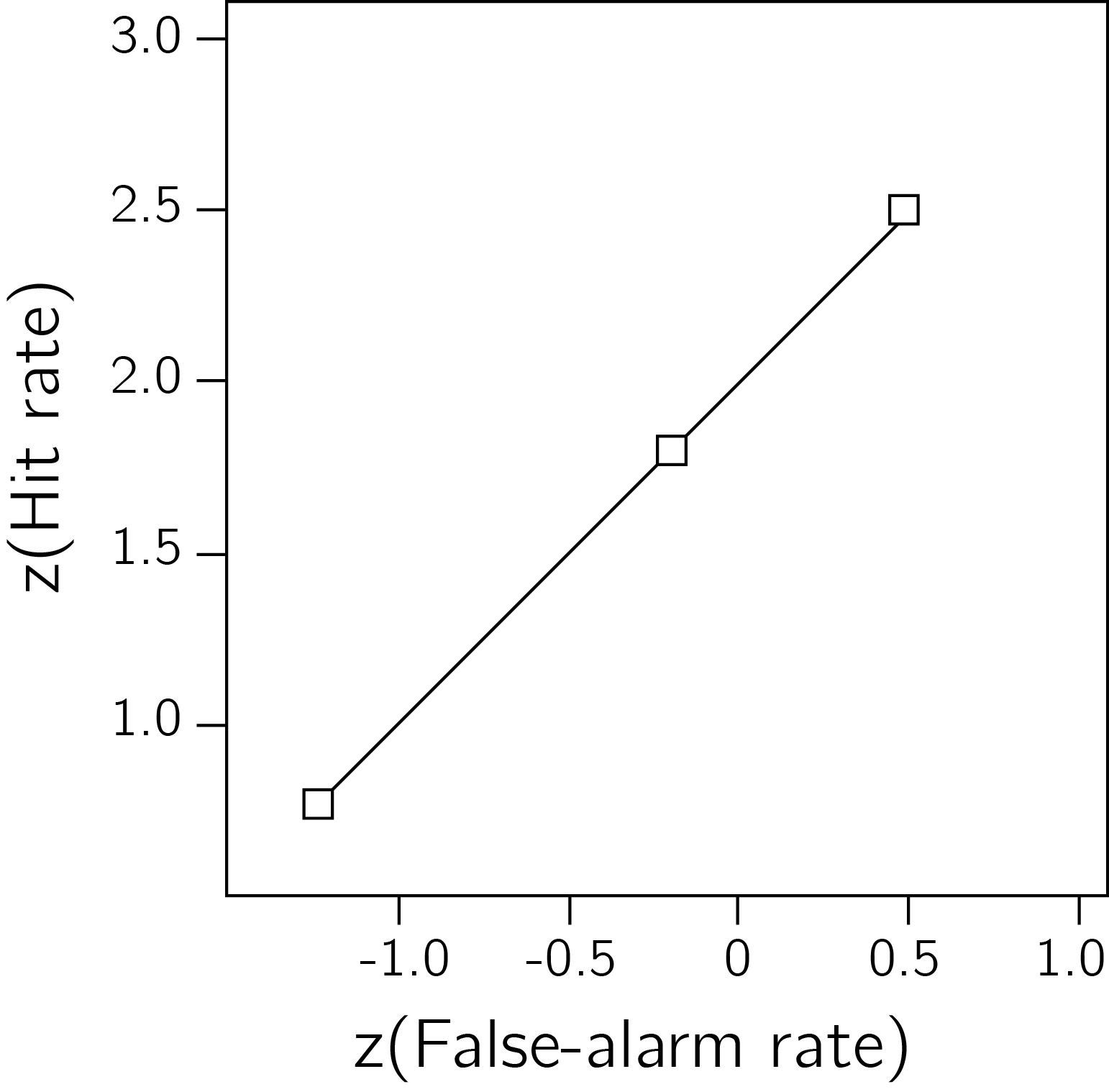
Figure A.3: zROC curve
A.2 Unequal-variance (uv) SDT
Unequal variance (uv) SDT can be applied to settings in which one distribution is assumed to be wider. For example, in perceptual detection tasks it is plausible that the signal distribution will be wider, as every sample comprises two sources of variance: a baseline noise component that is shared with the noise distribution, and the stimulus noise that represents fluctuations in the evidence strength available in the physical stimulus. A similar pattern is typically observed in recognition memory tasks.
This simple change to the model has profound effects on the decision making process. Under the assumption of equal-variance, the “log likelihood-ratio” (LLR; \(log(\frac{p(x|signal)}{p(x|noise)})\)) increases monotonically as a function of the decision variable, so that an optimal solution to the inference problem can rely on one decision criterion: samples to the right of the criterion are labeled as ‘signal,’ and samples to its left are labeled as ‘noise’ (Wickens, 2002, p. 30). The introduction of unequal variance to the SDT model makes inference more complex. Both extreme positive and extreme negative values are more likely to be drawn from the signal distribution when it is wider than the noise distribution, making a single-criterion decision rule sub-optimal. More specifically, in an unequal-variance setting, the LLR is proportional to the square of the decision variable. This means that it can be arbitrarily high for extremely positive or negative decision variables, but has a strict lower bound around the peak of the noise distribution.
A.3 SDT Measures for Metacognition
the ability to reliably track one’s objective performance in a perceptual or a memory task is commonly taken as a measure of one’s metacognitive ability (e.g., Fleming & Dolan, 2012). This ability can be quantified by asking participants for confidence judgments (“type-2 task”) following their primary decision (“type-1 task”). The match or mismatch between objective performance and confidence can then be used as a proxy for their “metacognitive sensitivity.”
The way this measure is extracted depends on the assumed underlying process. One potential process is a second-order SDT model, where a second variable is sampled following the type-1 decision, and this variable is then compared with an internal criterion that separates ‘confident’ responses from ‘unconfident’ responses (or a set of criteria, in the case of more than two possible confidence ratings). This variable is assumed to have higher values on average on trials in which the type-1 response was correct, similar to how the decision variable is higher on average on trials in which a signal is presented in a visual detection task (see figure A.4). Assuming that the two distributions of this confidence variable are normal, and assuming equal-variance, metacognitive sensitivity can then be quantified as the \(d'\) of the process that aims to separate between correct and incorrect responses . Alternatively, a type-2 ROC curve can be generated by plotting \(p(confidence>x|incorrect)\) against \(p(confidence>x|correct)\) for different values of x, and the area under this curve can be extracted as a measure of metacognitive sensitivity. Under these assumptions, these SDT measures have the desired properties of relative invariance of \(d'\) and AuROC to the positioning of the criterion and to performance level in the type-1 task (Kunimoto, Miller, & Pashler, 2001).
(ref:app1Kunimotocaption) A second order SDT model: confidence judgments are assumed to result from a process that uses an internal variable to separate correct from incorrect responses. Figure is based on Kunimoto, Miller, & Pashler, 2001.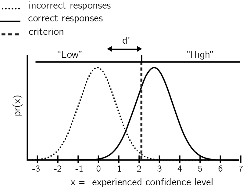
Figure A.4: (ref:ref:app1Kunimotocaption)
However, as discussed by Maniscalco & Lau (2012), this approach is unwarranted if the assumed underlying process uses the decision variable itself, or some transformation of it, in the generation of the confidence rating. In such a first-order model, the distance between the signal and noise distributions \(d'\) will be positively correlated with the estimated distance between the hypothetical ‘correct’ and ‘incorrect’ internal distributions. To correct for this, the authors propose to extract a measure of metacognitive sensitivity (\(meta-d'\)) that is fitted to the conditional distribution of confidence given stimulus and response, and compare it with \(d'\) (for example, by taking the ratio between these the two (\(M_{ratio}=meta-d'/d'\)). For an interactive primer on this approach, see matanmazor.shinyapps.io/sdtprimer.