3 Results

A summary of the results from all six experiments is available in section 3.7 and in Figures 3.1, 3.2 and 3.3.

3.1 Experiment 1: Q vs. O

In Experiment 1, we examined discrimination judgments between the two letters Q and O. Based on a search asymmetry for these letters (Qs are found faster than Os than vice-versa; Treisman and Souther 1985), we hypothesized that a similar asymmetry would emerge in subjective confidence judgments, such that metacognitive sensitivity for Q responses will be higher than for O responses. We used the letter Z as our backward mask.

205 participants were recruited from Prolific for Experiment 1.

Median completion time was 13.12 minutes. Mean accuracy was 0.74. Participants reported seeing an O on 0.47 of the trials. In a deviation from our pre-registration, we excluded 9 participants for having zero variance in their confidence ratings for at least one of the two responses (see Section 2.6). Overall we excluded 71 participants based on our exclusion criteria, leaving 134 participants for the main analysis. Due to a technical error in data collection, this figure is higher than that specified in our preregistration document (N=106). Going forward, only data from included participants is analyzed.

Mean accuracy among the included participants was \(M = 0.74\), 95% CI \([0.73\), \(0.75]\). Mean SOA in the last trial was \(M = 47.50\), 95% CI \([39.39\), \(55.61]\). Participants showed no consistent bias in their responses (quantified as the probability of a ‘Q’ response minus 0.5; \(M = 0.02\), 95% CI \([0.00\), \(0.04]\)). On a scale of 0 to 1, mean confidence level was \(M = 0.49\), 95% CI \([0.45\), \(0.53]\). Confidence was higher for correct than for incorrect responses (\(M_d = 0.15\), 95% CI \([0.13\), \(0.17]\), \(t(133) = 14.85\), \(p < .001\)).

Hypothesis 1: In line with our hypothesis, confidence was generally higher for Q (feature present) responses than for O (feature absent) responses (\(t(133) = 7.52\), \(p < .001\); Cohen’s d = 0.65; \(\mathrm{BF}_{\textrm{10}} = 1.07 \times 10^{9}\); see Fig. 3.1, panel 1).

Hypothesis 2: In order to measure metacognitive asymmetry, we extracted the response-conditional type-2 ROC (rc-ROC) curves for the two responses (Q and O) in the discrimination task. This was done by plotting the cumulative distribution of confidence ratings (high to low) for correct responses against the same distribution for incorrect responses. The area under the rc-ROC curve (auROC) was then taken as a measure of metacognitive sensitivity (Kanai, Walsh, and Tseng 2010; Meuwese et al. 2014). In line with our hypothesis, auROC for Q responses (\(M = 0.72\), 95% CI \([0.70\), \(0.74]\)) was higher than for O responses (\(M = 0.68\), 95% CI \([0.66\), \(0.70]\); \(t(133) = 2.96\), \(p = .002\); Cohen’s d = 0.26; \(\mathrm{BF}_{\textrm{10}} = 6.56\); see Figure 3.2, panel 1), similar to the documented metacognitive asymmetry for detection judgments.

Hypothesis 3: Metacognitive asymmetry was not significantly higher than what is expected based on an equal-variance SDT model with the same response bias and sensitivity as the subjects (\(t(133) = 0.97\), \(p = .167\); Cohen’s d=0.08). A Bayes Factor indicated that our results are more likely under a model that assumes no additional metacognitive asymmetry (\(\mathrm{BF}_{\textrm{01}} = 6.07\)).

Hypothesis 4: In line with our hypothesis, Q responses were faster on average than O responses by 37 ms. (\(t(133) = -2.99\), \(p = .002\) ; Cohen’s d = 0.26; \(\mathrm{BF}_{\textrm{10}} = 7.05\); see Fig. 3.1, panel 1).

In summary, in Experiment 1 we found that Q responses were faster and accompanied by higher subjective confidence, in line with a processing advantage for feature-presence. Metacognitive asymmetry however did not go beyond what is expected from an equal-variance SDT model for these stimuli, taking into account response biases.

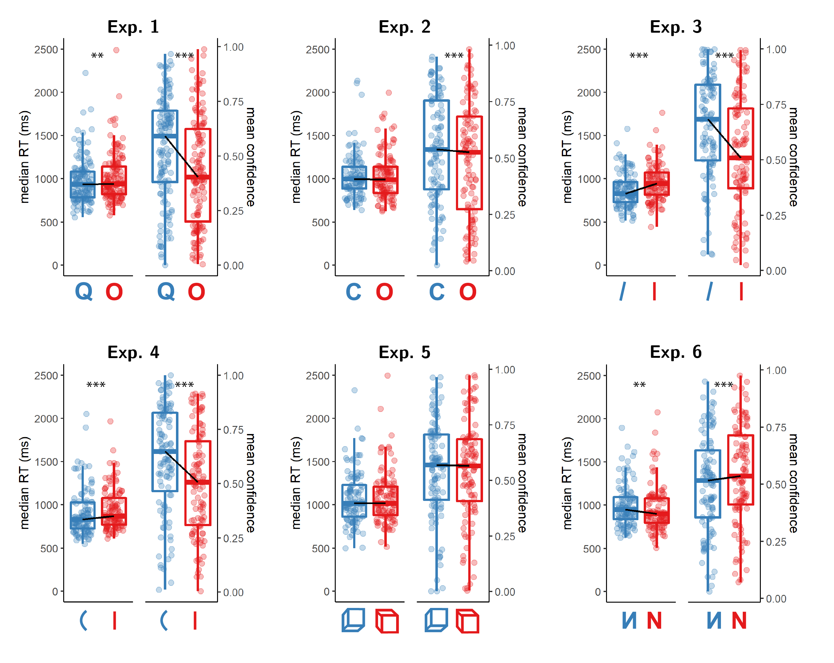
Figure 3.1: Reaction time and confidence distributions for Experiments 1-6. Box edges and central lines represent the 25, 50 and 75 quantiles. Whiskers cover data points within four inter-quartile ranges around the median. Black lines connect the median values for the two responses. Stars represent significance in a two-sided t-test: **: p<0.01, ***: p<0.001

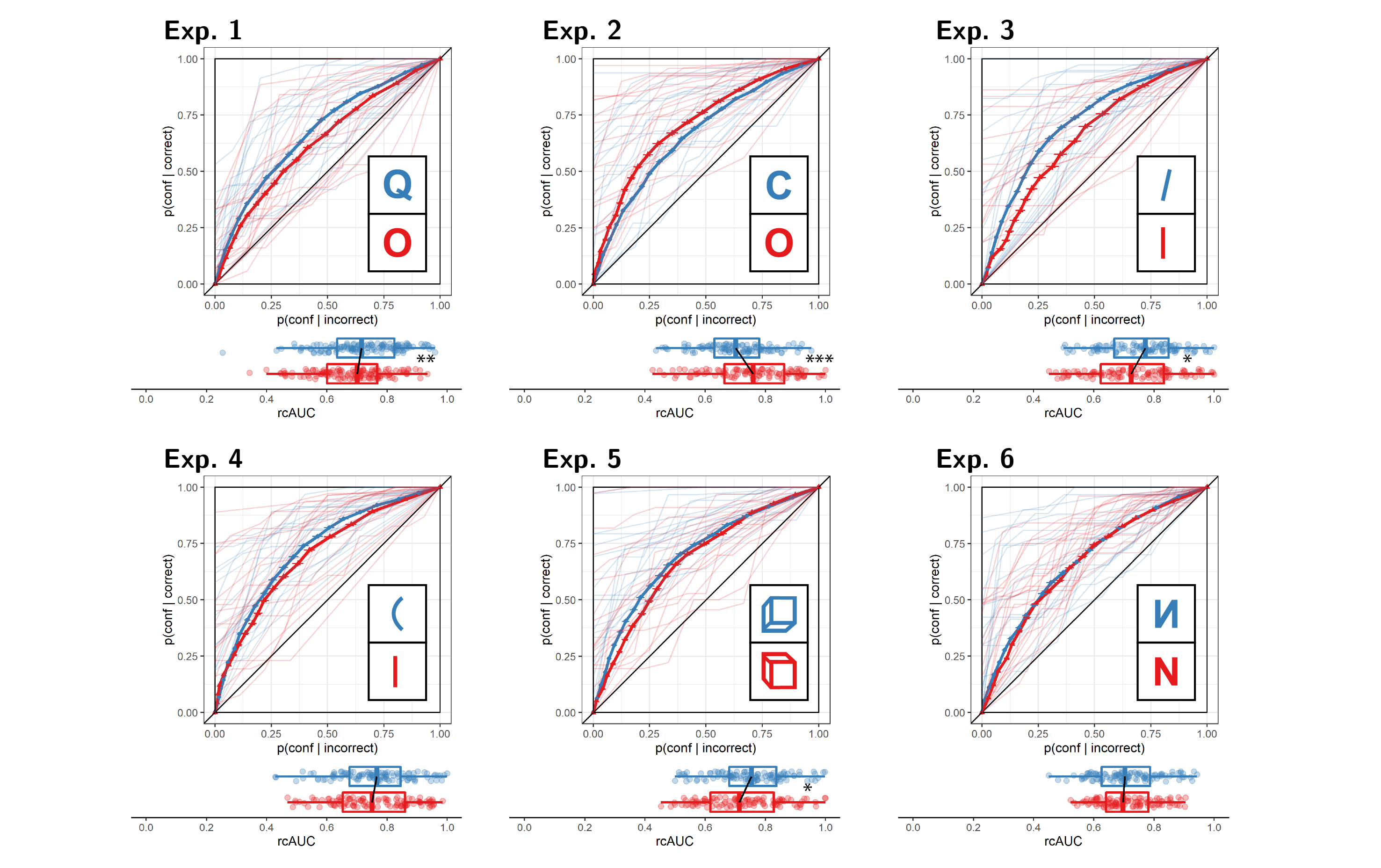
Figure 3.2: Response conditional ROC curves for Experiments 1-6. The area under the curve is a measure of metacognitive sensitivity. Error bars stand for the standard error of the mean. For illustration, the response-conditional ROC curves of the first 20 participants of each Experiment are plotted in low opacity. Below each ROC: distributions of the area under the curve for the two responses, across participants. Same conventions as Fig. 3.1. Stars represent significance in a two-sided t-test: *: p<0.05, **: p<0.01, ***: p<0.001

3.2 Experiment 2: C vs. O

In Experiment 2, we examined discrimination judgments between the two letters C and O. Based on a search asymmetry for these letters (Cs are found faster among Os than vice versa; Treisman and Souther 1985; Takeda and Yagi 2000; Treisman and Gormican 1988), we hypothesized that a similar asymmetry would emerge in subjective confidence judgments, such that metacognitive sensitivity for perceiving a C will be higher than for perceiving an O. We used the letter Z as our backward mask.

143 participants were recruited from Prolific for Experiment 2.

Median completion time was 12.80 minutes. Mean accuracy was 0.75, and participants reported seeing an O on 0.43 of the trials. In a deviation from our pre-registration, we excluded 8 participants for having zero variance in their confidence ratings for at least one of the two responses (see Section 2.6). Overall we excluded 37 participants, leaving 106 participants for the main analysis. Going forward, only data from included participants is analyzed.

Mean accuracy among included participants was \(M = 0.74\), 95% CI \([0.73\), \(0.75]\). The mean SOA of the last trial was \(M = 40.18\), 95% CI \([34.37\), \(46.00]\). Participants showed a consistent bias toward reporting a C rather than an O (\(M = 0.07\), 95% CI \([0.05\), \(0.08]\)). On a scale of 0 to 1, mean confidence level was \(M = 0.52\), 95% CI \([0.48\), \(0.56]\). Confidence was higher for correct than for incorrect responses (\(M_d = 0.17\), 95% CI \([0.15\), \(0.19]\), \(t(105) = 15.05\), \(p < .001\)).

Hypothesis 1: In line with our hypothesis, confidence was generally higher for C (feature present) responses than for O (feature absent) responses (\(M_d = 0.05\), 95% CI \([0.03\), \(\infty]\), \(t(105) = 3.59\), \(p < .001\); Cohen’s d = 0.35; \(\mathrm{BF}_{\textrm{10}} = 42.62\); see Figure 3.2, panel 2).

Hypothesis 2: Opposite to our prediction, auROC for C responses (\(M = 0.70\), 95% CI \([0.68\), \(0.72]\)) was lower than for O responses (\(M = 0.75\), 95% CI \([0.73\), \(0.78]\); \(t(105) = -3.53\), \(p > .999\); Cohen’s d = 0.34; see Figure 3.2, panel 2.). Bayes Factor strongly supported the alternative (\(\mathrm{BF}_{\textrm{10}} = 35.19\)). Note that our prior on effect sizes was symmetric around zero, such that support for the alternative is obtained for negative, as well as positive effects.

Hypothesis 3: Metacognitive sensitivity for C responses was still higher than for O responses after controlling for bias (Cohen’s d=0.49; \(\mathrm{BF}_{\textrm{10}} = 6.46 \times 10^{3}\)).

Hypothesis 4: Contrary to our hypothesis, response times for C and for O responses were highly similar, with a median difference of 6 ms. (\(t(105) = 0.01\), \(p = .504\) ; Cohen’s d = 0.00; \(\mathrm{BF}_{\textrm{01}} = 8.57\); see Figure 3.2, panel 2).

In summary, in Experiment 2 we found a dissociation between our two confidence-related measures. As we hypothesized, participants were generally more confident in their C (feature present) responses, but their metacognitive sensitivity was higher following O (feature absent) responses. We found no reliable difference in response times between these two responses.

3.3 Experiment 3: tilted vs. vertical lines

In Experiment 3, we examind discrimination judgments between tilted and vertical lines. Based on a search asymmetry for these stimuli (tilted lines are found faster among vertical lines than vice versa; Treisman and Gormican 1988), we hypothesized that a similar asymmetry would emerge in subjective confidence judgments, such that metacognitive sensitivity for perceiving a tilted line will be higher than for perceiving a vertical line. As described in section 2.6, overly high accuracy in the first few participants led us to change our masking stimulus, first to an overlay of all stimuli and then to four dollar signs. We present here the combined results from these last two cohorts of participants (94 and 210 participants, respectively). The results were qualitatively similar in the two cohorts.

304 participants were recruited from Prolific for Experiment 3. Due to shorter than expected completion times in the first 94 participants, the remaining participants were paid £1.25, equivalent to an hourly wage of £6.

Median completion time was 12.43 minutes. Mean accuracy was 0.86, and participants reported seeing a vertical line on 0.44 of the trials. In a deviation from our pre-registration, we excluded 14 participants for having zero variance in their confidence ratings for at least one of the two responses (see Section 2.6). Overall we excluded 198 participants, leaving 106 participants for the main analysis. Going forward, only data from included participants is analyzed.

Mean accuracy among included participants was \(M = 0.79\), 95% CI \([0.78\), \(0.81]\). The mean SOA of the last trial was \(M = 30.83\), 95% CI \([25.99\), \(35.68]\). Participants showed a consistent bias toward reporting a tilted rather than a vertical line (\(M = 0.06\), 95% CI \([0.04\), \(0.08]\)). On a scale of 0 to 1, mean confidence level was \(M = 0.61\), 95% CI \([0.56\), \(0.65]\). Confidence was higher for correct than for incorrect responses (\(M_d = 0.18\), 95% CI \([0.15\), \(0.20]\), \(t(105) = 13.42\), \(p < .001\)).

Hypothesis 1: In line with our hypothesis, confidence was generally higher for tilted lines (feature present) responses than for vertical lines (feature absent) responses (\(M_d = 0.12\), 95% CI \([0.09\), \(\infty]\), \(t(105) = 7.18\), \(p < .001\); Cohen’s d = 0.70; \(\mathrm{BF}_{\textrm{10}} = 8.89 \times 10^{7}\); see Figure 3.2, panel 3).

Hypothesis 2: Contrary to our prediction, Bayes Factor analysis did not provide evidence for or against a difference in auROC between reports of seeing a tilted line (\(M = 0.76\), 95% CI \([0.74\), \(0.78]\)) and reports of seeing a vertical line (\(M = 0.73\), 95% CI \([0.70\), \(0.75]\); Cohen’s d = 0.18; \(\mathrm{BF}_{\textrm{01}} = 1.59\); see Figure 3.2, panel 3.). A difference in metacognitive sensitivity was however significant in a standard t-test (\(t(105) = 1.88\), \(p = .031\)). With a sample size of 106, a one-tailed t-test is significant for observed effect sizes of 0.16 standard deviations or higher. In contrast, for our choice of a scale factor, a Bayes Factor is higher than 3 for observed standardized effect sizes of \(0.26\) standard deviations or higher. Effect sizes that fall between 0.16 and \(0.26\) are then significant in a t-test, with no conclusive evidence in a Bayes Factor analysis. A robustness region analysis revealed that no scale factor would have led to the conclusion that auROCs for the two responses are different with \(BF_{10}>3\). See Supplementary Figure A.1 for a full Robustness Region plot (Dienes 2019).

Hypothesis 3: A Bayes Factor analysis did not provide evidence for or against metacognitive asymmetry when controlling for response bias and sensitivity (\(t(105) = -0.70\), \(p = .759\); Cohen’s d=0.07; \(\mathrm{BF}_{\textrm{01}} = 6.74\)).

Hypothesis 4: In line with our hypothesis, response times for ‘tilted’ responses were faster than response times for ‘vertical’ responses, with a median difference of 68 ms. (\(t(105) = -5.82\), \(p < .001\) ; Cohen’s d = 0.56; \(\mathrm{BF}_{\textrm{10}} = 1.83 \times 10^{5}\); see Figure 3.2, panel 3).

In summary, in Experiment 3 we found that ‘tilted’ (feature present) responses were faster and accompanied by higher subjective confidence that ‘vertical’ (feature absent) responses, with no difference in metacognitive sensitivity between the two responses.

3.4 Experiment 4: curved vs. straight lines

In Experiment 4, we examined discrimination judgments between curved and vertical lines. Based on a search asymmetry for these stimuli (curved lines are found faster among vertical lines than vice versa; Treisman and Gormican 1988), we hypothesized that a similar asymmetry would emerge in subjective confidence judgments, such that metacognitive sensitivity for perceiving a tilted line will be higher than for perceiving a vertical line. We used four dollar signs as our mask.

211 participants were recruited from Prolific for Experiment 4. Due to shorter than expected completion times in previous experiments, participants were paid £1.25, equivalent to an hourly wage of £6.

Median completion time was 12.08 minutes. Mean accuracy was 0.84, and participants reported seeing a straight line on 0.44 of the trials. In a deviation from our pre-registration, we excluded 11 participants for having zero variance in their confidence ratings for at least one of the two responses (see Section 2.6). Overall we excluded 104 participants, leaving 107 participants for the main analysis. Going forward, only data from included participants is analyzed.

Mean accuracy among included participants was \(M = 0.79\), 95% CI \([0.77\), \(0.80]\). The mean SOA of the last trial was \(M = 28.01\), 95% CI \([24.22\), \(31.79]\). Participants showed a consistent bias toward reporting a curved rather than a vertical line (\(M = 0.06\), 95% CI \([0.04\), \(0.07]\)). On a scale of 0 to 1, mean confidence level was \(M = 0.57\), 95% CI \([0.53\), \(0.61]\). Confidence was higher for correct than for incorrect responses (\(M_d = 0.21\), 95% CI \([0.18\), \(0.24]\), \(t(106) = 14.96\), \(p < .001\)).

Hypothesis 1: In line with our hypothesis, confidence was generally higher for curved lines (feature present) responses than for straight lines (feature absent) responses (\(M_d = 0.12\), 95% CI \([0.09\), \(\infty]\), \(t(106) = 8.25\), \(p < .001\); Cohen’s d = 0.80; \(\mathrm{BF}_{\textrm{10}} = 1.61 \times 10^{10}\); see Figure 3.2, panel 4).

Hypothesis 2: Contrary to our prediction, auROC for reports of seeing a curved line (\(M = 0.76\), 95% CI \([0.73\), \(0.78]\)) was similar to auROC for reports of seeing a straight line (\(M = 0.75\), 95% CI \([0.73\), \(0.78]\); \(t(106) = 0.30\), \(p = .382\); Cohen’s d = 0.03; \(\mathrm{BF}_{\textrm{01}} = 8.23\); see Figure 3.2, panel 4.).

Hypothesis 3: (The lack of) metacognitive asymmetry was not different from what would be expected based on an equal-variance SDT model with the same response bias and sensitivity (\(t(106) = -1.93\), \(p = .972\); Cohen’s d=0.19; \(\mathrm{BF}_{\textrm{01}} = 1.45\)).

Hypothesis 4: In line with our hypothesis, response times for ‘curved’ responses were faster than response times for ‘straight’ responses, with a median difference of 51 ms (\(t(106) = -4.36\), \(p < .001\) ; Cohen’s d = 0.42; \(\mathrm{BF}_{\textrm{10}} = 558.55\); see Figure 3.2, panel 4).

In summary, similar to Experiment 3, ‘curved’ (feature-present) responses were faster and accompanied by higher subjective confidence than ‘straight’ (feature absent) responses. However, similar to the results of Experiment 3, here also we did not find a metacognitive asymmetry for these stimuli.

3.5 Experiment 5: upward-tilted vs. downward-tilted cubes

In Experiment 5, we examined discrimination judgments between upward-tilted and downward-tilted cubes. Based on a search asymmetry for these stimuli (upward-tilted cubes are found faster among downward-tilted cubes than vice versa, in line with an expectation to see objects on the ground and not floating in space; Von Grünau and Dubé 1994), we hypothesized that a similar asymmetry would emerge in subjective confidence judgments, such that metacognitive sensitivity for perceiving an upward-tilted cube will be higher than for perceiving a downward-tilted cube. We used four dollar signs as our mask.

162 participants were recruited from Prolific for Experiment 5.

Median completion time was 13.30 minutes. Mean accuracy was 0.79, and participants reported seeing a downward-tilted cube on 0.51 of the trials. In a deviation from our pre-registration, we excluded 11 participants for having zero variance in their confidence ratings for at least one of the two responses (see Section 2.6). Overall we excluded 56 participants, leaving 106 participants for the main analysis. Going forward, only data from included participants is analyzed.

Mean accuracy among included participants was \(M = 0.77\), 95% CI \([0.76\), \(0.78]\). The mean SOA of the last trial was \(M = 29.51\), 95% CI \([23.20\), \(35.81]\). Participants showed no consistent response bias (\(M = -0.01\), 95% CI \([-0.03\), \(0.00]\)). On a scale of 0 to 1, mean confidence level was \(M = 0.55\), 95% CI \([0.51\), \(0.59]\). Confidence was higher for correct than for incorrect responses (\(M_d = 0.23\), 95% CI \([0.20\), \(0.26]\), \(t(105) = 13.89\), \(p < .001\)).

Hypothesis 1: Contrary to our hypothesis, confidence was similar for upward-tilted (feature present) responses and downward-tilted (feature absent) responses (\(M_d = 0.00\), 95% CI \([-0.02\), \(\infty]\), \(t(105) = 0.12\), \(p = .452\); Cohen’s d = 0.01; \(\mathrm{BF}_{\textrm{01}} = 8.51\); see Figure 3.2, panel 5).

Hypothesis 2: Contrary to our hypothesis, A Bayes Factor analysis did not provide evidence for or against a difference in auROC for reports of seeing an upward-tilted cube (\(M = 0.75\), 95% CI \([0.73\), \(0.77]\)) and reports of seeing a downward-tilted cube (\(M = 0.72\), 95% CI \([0.70\), \(0.75]\); Cohen’s d = 0.22; \(\mathrm{BF}_{\textrm{10}} = 1.38\); see Figure 3.2, panel 5.). In contrast, a t-test revealed a significant metacognitive asymmetry, with higher metacognitive sensitivity for perceiving an upward-tilted (default-violating) cube (\(t(105) = 2.29\), \(p = .012\)). See Supplementary Figure A.1 for a full Robustness Region plot (Dienes 2019).

Hypothesis 3: (The lack of) metacognitive asymmetry was not different from what would be expected based on an equal-variance SDT model with the same response bias and sensitivity (Cohen’s d=0.22; \(\mathrm{BF}_{\textrm{10}} = 1.28\)). Here also, frequentist and Bayesian analyses conflicted, with a t-test revealing a significant metacogntiive advantage for upward-tilted (default violating) responses when controlling for bias (\(t(105) = 2.25\), \(p = .013\)).

Hypothesis 4: Contrary to our hypothesis, response times for ‘upward-tilted’ responses were similar to response times for ‘downward-tilted’ responses with a median difference of 9 ms. (\(t(105) = -0.82\), \(p = .207\) ; Cohen’s d = 0.08; \(\mathrm{BF}_{\textrm{01}} = 6.19\); see Figure 3.2, panel 5).

In summary, in Experiment 5 we found no sign of processing asymmetry between upward and downward-tilted cubes in response-times and confidence. A significant metacognitive asymmetry was observed when using null-hypothesis significance testing, but was not supported by our Bayes Factor analysis. In accordance with our pre-registered plan to commit to the Bayes Factor analysis in interpreting the results, in what follows we interpret these findings as providing no support for a metacognitive asymmetry for upward and downward tilted cubes.

3.6 Experiment 6: flipped vs. normal letters

In Experiment 6, we examined discrimination judgments between flipped and normal N stimuli. Based on a search asymmetry for these stimuli (flipped Ns are found faster among normal Ns than vice versa; Frith 1974; Wang, Cavanagh, and Green 1994), we hypothesized that a similar asymmetry would emerge in subjective confidence judgments, such that metacognitive sensitivity for perceiving a flipped N will be higher than for perceiving a normal N. We used four dollar signs as our mask.

127 participants were recruited from Prolific for Experiment 6. Due to shorter than expected completion times in previous experiments, participants were paid £1.25, equivalent to an hourly wage of £6.

Median completion time was 12.76 minutes. Mean accuracy was 0.74, and participants reported seeing a normal N on 0.50 of the trials. In a deviation from our pre-registration, we excluded 4 participants for having zero variance in their confidence ratings for at least one of the two responses (see Section 2.6). Overall we excluded 21 participants, leaving 106 participants for the main analysis. Going forward, only data from included participants is analyzed.

Mean accuracy among included participants was \(M = 0.73\), 95% CI \([0.72\), \(0.74]\). The mean SOA in the last trial was \(M = 37.26\), 95% CI \([33.07\), \(41.46]\). Participants showed no consistent response bias (\(M = 0.00\), 95% CI \([-0.02\), \(0.02]\)). On a scale of 0 to 1, mean confidence level was \(M = 0.53\), 95% CI \([0.49\), \(0.57]\). Confidence was higher for correct than for incorrect responses (\(M_d = 0.17\), 95% CI \([0.15\), \(0.20]\), \(t(105) = 16.45\), \(p < .001\)).

Hypothesis 1: Contrary to our hypothesis, confidence was lower for flipped (feature present) responses than for normal (feature absent) responses. This result was in the opposite direction to what we had expected, so was not significant in a one-tailed t-test (\(M_d = -0.04\), 95% CI \([-0.06\), \(\infty]\), \(t(105) = -3.32\), \(p = .999\); Cohen’s d = 0.32). However, a Bayes Factor favoured the alternative over the null (\(\mathrm{BF}_{\textrm{10}} = 18.92\); see Figure 3.2, panel 6).

Hypothesis 2: Contrary to our hypothesis, auROC for reports of seeing a flipped N (\(M = 0.71\), 95% CI \([0.69\), \(0.73]\)) was similar to auROC for reports of seeing a normal N (\(M = 0.71\), 95% CI \([0.69\), \(0.73]\); \(t(105) = 0.08\), \(p = .468\); Cohen’s d = 0.01; \(\mathrm{BF}_{\textrm{01}} = 8.54\); see Figure 3.2, panel 6.).

Hypothesis 3: (The lack of) metacognitive asymmetry was not different from what would be expected based on an equal-variance SDT model with the same response bias and sensitivity (\(t(105) = 0.26\), \(p = .396\); Cohen’s d=0.03; \(\mathrm{BF}_{\textrm{01}} = 8.28\)).

Hypothesis 4: Contrary to our hypothesis, response times for ‘flipped’ responses were slower than response times for ‘normal’ responses, with a median difference of 30 ms. (\(t(105) = 2.81\), \(p = .997\) ; Cohen’s d = 0.27; \(\mathrm{BF}_{\textrm{10}} = 4.66\); see Figure 3.2, panel 6).

In summary, in Experiment 6 we found a difference in response speed and subjective confidence in the opposite direction to what we expected, with a processing advantage for the default-complying stimulus (N) compared to the default-violating stimulus (flipped N). We found no metacognitive asymmetry for these stimuli.

3.7 Experiments 1-6: summary

Overall, the pattern of results from Experiments 1-6 only partly matched our hypotheses in some cases, and stood in direct contrast to them in other cases (see fig. 3.3). A reliable metacognitive asymmetry was observed only in Experiment 2, and this asymmetry was in the opposite direction to what we had predicted, with a metacognitive advantage for O (feature absent) over C (feature present) responses. A metacognitive advantage for reporting Q over Os (Exp. 1) was not reliably above what is expected based on an equal-variance signal detection model.

For both local and global visual features (Experiments 1-4) we observed differences in mean confidence and response times that were consistent with our hypothesis of a processing advantage for the representation of the presence compared to the absence of visual features. In Experiments 5 and 6, we tested more abstract expectation violations. In Experiment 5, discrimination between upward-tilted and downward-tilted cubes showed no asymmetry in response time and confidence. In Experiment 6, participants were less confident and slower in their reports of seeing a flipped N, contrary to our prediction that default-violating signals should be easier to perceive. We found no evidence for or against a metacognitive sensitivity in either of the experiments.

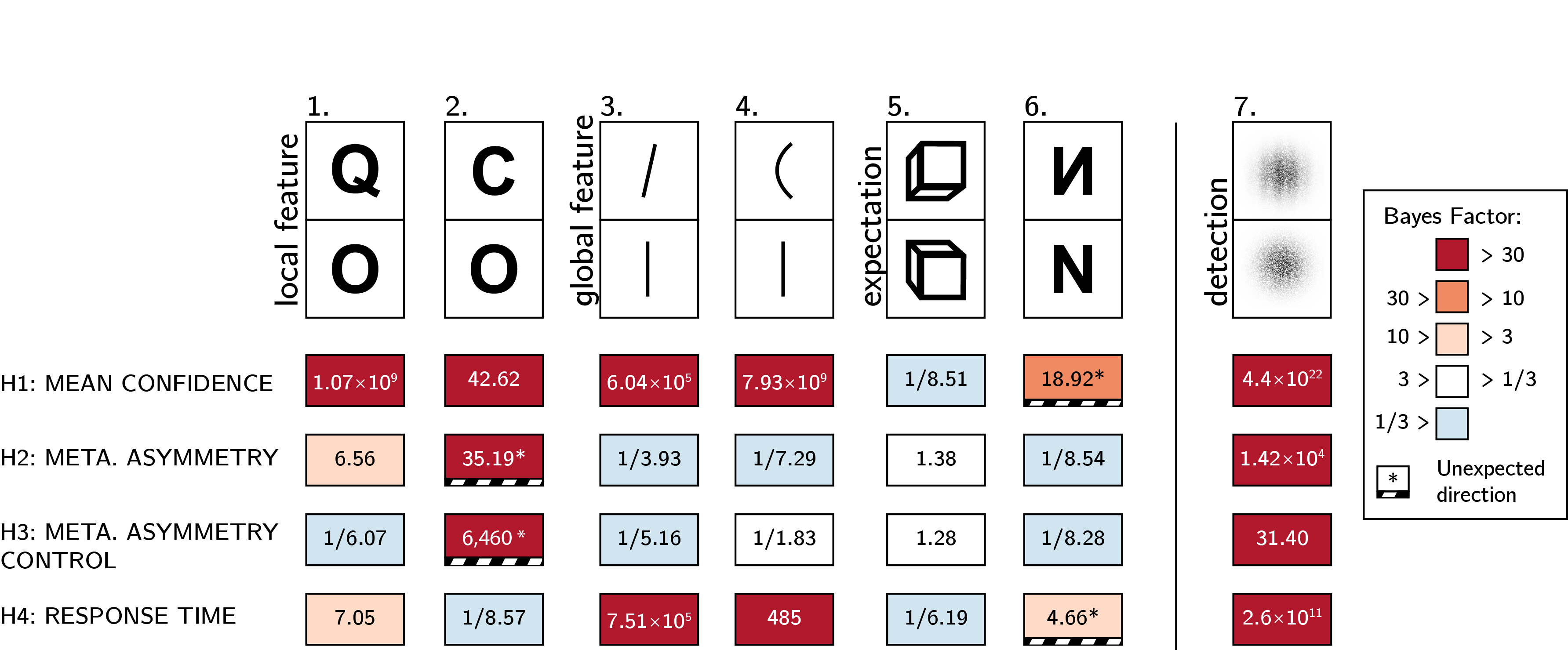
Figure 3.3: Summary of results from Experiments 1-6, and exploratory Experiment 7. Rows correspond to our four pre-registered hypotheses: difference in confidence, a difference in metacognitive sensitivity, a difference in metacognitive sensitivity when controlling for response and confidence bias, and a difference in response times.

3.8 Experiment 7 (exploratory): grating vs. noise

Results from Experiments 1-6 revealed that search asymmetry is not always accompanied by an asymmetry in metacognitive sensitivity. Given that we did not observe a true metacognitive asymmetry in the expected direction for any of our stimulus pairs, we were concerned that our experimental design may have been unsuitable for detecting classical metacognitive asymmetries in detection, for example due to an insufficient number of trials, the masking procedure, or the confidence report scheme. As a positive control, we collected data for an additional experiment that more closely resembled typical detection experiments. In this experiment, participants discriminated between two stimuli: random noise and a noisy grating (presented to participants as a ‘zebra’ stimulus; see Fig. 3.4). In a previous lab-based study, similar stimuli produced a robust metacognitive asymmetry between target absent (noise) and target present (noisy grating) responses (Mazor, Friston, and Fleming 2020). We used black and white concentric circles as a mask. Apart from the choice of stimuli and mask, the procedure was identical to that of our pre-registered experiments.

127 participants were recruited from Prolific for exploratory Experiment 7. For this positive control, all four hypotheses were fulfilled.

Median completion time was 10.70 minutes. Mean accuracy was 0.73, and participants reported seeing a grating on 0.48 of the trials. Overall we excluded 36 participants, leaving 105 participants for the main analysis. Going forward, only data from included participants is analyzed.

Mean accuracy among included participants was \(M = 0.76\), 95% CI \([0.74\), \(0.77]\). The mean SOA of the last trial was \(M = 53.87\), 95% CI \([38.85\), \(68.89]\). Participants showed no consistent response bias (\(M = 0.01\), 95% CI \([0.00\), \(0.03]\)). On a scale of 0 to 1, mean confidence level was \(M = 0.55\), 95% CI \([0.51\), \(0.59]\). Confidence was higher for correct than for incorrect responses (\(M_d = 0.15\), 95% CI \([0.13\), \(0.17]\), \(t(104) = 12.58\), \(p < .001\)).

Hypothesis 1: In line with our hypothesis, confidence was higher for reports of target presence than for reports of target absence (\(M_d = 0.20\), 95% CI \([0.17\), \(\infty]\), \(t(104) = 14.07\), \(p < .001\); Cohen’s d = 1.37; \(\mathrm{BF}_{\textrm{10}} = 4.39 \times 10^{22}\); see Figure 3.4, right panel).

Hypothesis 2: In line with our hypothesis, auROC for reports of target presence (\(M = 0.75\), 95% CI \([0.73\), \(0.77]\)) was higher than for reports of target absence (\(M = 0.68\), 95% CI \([0.66\), \(0.70]\); \(t(104) = 5.20\), \(p < .001\); Cohen’s d = 0.51; \(\mathrm{BF}_{\textrm{10}} = 1.42 \times 10^{4}\); see Figure 3.4, left panel).

Hypothesis 3: In line with our hypothesis, this metacognitive asymmetry was stronger than what is expected based on an equal-variance SDT model with the same response bias and sensitivity (\(t(104) = 3.49\), \(p < .001\); Cohen’s d=0.34; \(\mathrm{BF}_{\textrm{10}} = 31.40\)).

Hypothesis 4: In line with our hypothesis, reports of target presence were faster than reports of target absence, with a median difference of 124 ms. (\(t(104) = -8.84\), \(p < .001\) ; Cohen’s d = 0.86; \(\mathrm{BF}_{\textrm{10}} = 2.63 \times 10^{11}\); see Figure 3.4, right panel).

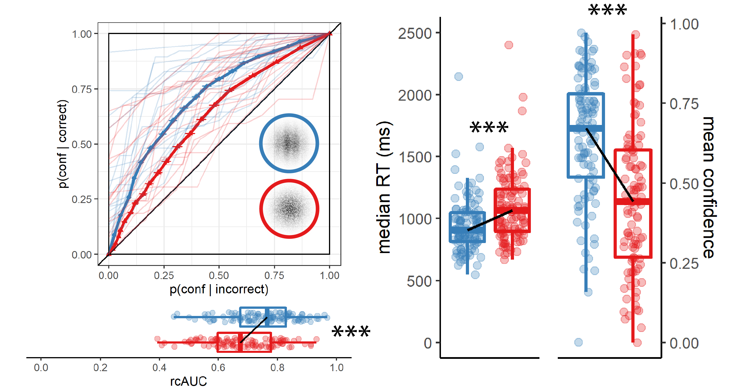
Figure 3.4: Response conditional ROC curves (left panel) and confidence and reaction time distributions (right panel) for Exp. 7 (detection positive control). The structure of this figure is similar to Figs 3-4.

3.9 Exploratory analysis

3.9.1 zROC analysis

In a signal-detection framework, metacognitive asymmetry appears when the signal distribution has both a higher mean and higher variance than that of the noise distribution. This unequal variance setting produces higher metacognitive sensitivity for judgments of signal presence, compared to judgments of signal absence. A direct measure for the ratio between the variances of the two distributions is the slope of the type-1 zROC curve. A zROC curve is constructed by applying the inverse of the normal cumulative density function to false alarm and hit rates for different confidence thresholds. The slope of the zROC curve equals 1 exactly when the variance of the signal and noise distributions are equal. In detection experiments, the slope is often shallower than 1, indicating a wider signal distribution. Indeed, in our positive control experiment (Exp. 7), the median zROC slope was 0.86 and significantly shallower than 1 (\(t(103) = -5.08\), \(p < .001\) for a t-test on the log-slope against zero). Measuring the slope of the zROC curve in our six pre-registered experiments, we asked whether our ‘feature-present’ distributions had higher variance than our ‘feature-absent’ distributions. We used the standardized effect size obtained from Experiment 7 as a scaling factor for the prior distribution over effect sizes, reflecting a belief that a difference in slopes should be similar in magnitude to what is observed in a detection task.

zROC slopes were numerically shallower than one in Experiments 1 (Q vs. O; median slope = 0.95), 3 (line tilt; median slope = 0.94), 4 (line curvature; 0.97) and 5 (cube orientation; 0.95). This was significant only in Experiment 5 (\(t(101) = -2.09\), \(p = .039\)). In agreement with the results of our rcROC analysis, the zROC slope in Exp. 2 (C vs. O) was significantly higher than one, suggesting that the representation of the letter ‘O’ was more variable than that of the letter ‘C’ (median slope = 1.09; \(t(104) = 2.29\), \(p = .024\)). A Bayes Factor analysis did not provide support for or against the null hypothesis for any of the six experiments (all Bayes Factors between 1/3 and 3).

Previous studies reported similar variance structures for these stimuli when presented in visual search arrays. For example, confidence in a vertical/tilted visual search task revealed higher variance in the representation of tilted (feature positive) compared to vertical (feature negative) stimuli (Vincent 2011). Similarly, reverse correlation analysis revealed higher variance in the representation of Q (feature positive) compared to O (feature negative) stimuli (Saiki 2008). Finally, and in agreement with our results, variance in the representation of O (feature negative) was found to be higher than in the representation of C (feature positive) (Dosher, Han, and Lu 2004). Note that for the case of line tilt and Q vs. O, finding a high-variance target among low-variance distractors is easier than finding a low-variance target among high-variance distractors. However, the opposite is true for C vs. O, where a low-variance target (C) renders the search easier. This last observation challenges the suggestion that variance structure is the determining factor for visual search asymmetries (Treisman and Gormican 1988; Dosher, Han, and Lu 2004; Vincent 2011; Saiki 2008).

3.9.2 Inter-subject correlations

Across experiments, asymmetry in mean confidence (Hypothesis 1) and in response time (Hypothesis 4) were mostly aligned. This is consistent with previous reports of a negative correlation between response times and confidence across trials within participants (Henmon 1911; Calder-Travis et al. 2020; Pleskac and Busemeyer 2010; Moran, Teodorescu, and Usher 2015). To test if this was the case across participants too, and not only across experiments, we fitted a mixed-effects regression model to data from all seven experiments with experiment as a random effect (\(\Delta RT \sim \Delta conf+(1+\Delta conf|exp)\)). The association between confidence and RT effects was significant in this model (\(p<0.001\); see Fig. 3.5; upper panel). In contrast, metacognitive asymmetry (difference between the area under the response conditional ROC curves, controlling for response bias) was not significantly associated with asymmetry in either confidence ratings (\(p=0.41\); see Fig. 3.5; lower panel) or reaction time (\(p=0.54\)).

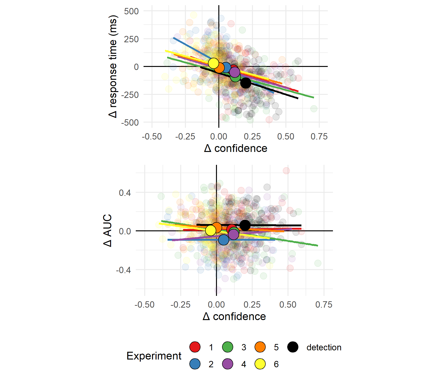
Figure 3.5: Upper panel: Difference in mean confidence between S1 and S2 responses plotted against difference in mean response time between S1 and S2 responses across the seven experiments. Lower panel: Difference in mean confidence between S1 and S2 responses plotted against difference in metacognitive sensitivity, controlling for response bias, across the seven experiments. Semi-transparent circles represent individual subjects. Opaque circles are the means for each of the seven experiments, across participants. Lines indicate the best-fitting linear regression line for experiments 1-7.