2 Methods
We report how we determined our sample size, all data exclusions (if any), all manipulations, and all measures in the study. The full registered protocol is available at osf.io/ed8n7.
We ran six experiments, that were identical except for the identity of the two stimuli \(S_1\) and \(S_2\) (and of the stimulus used for backward masking; see section 2.6 for details). Our choice of stimuli for this study was based on the visual search literature. For some stimulus pairs \(S_1\) and \(S_2\), searching for one \(S_1\) among multiple \(S_2\)s is more efficient than searching for one \(S_2\) among multiple \(S_1\)s. Such search asymmetries have been reported for stimulus pairs that are identical except for the presence and absence of a distinguishing feature. Importantly, distinguishing features vary in their level of abstraction, from concrete local features (finding a Q among Os is easier than the inverse search; Treisman and Souther 1985), through global features (finding a curved line among straight lines is easier than the inverse search; Treisman and Gormican 1988), and up to the presence or absence of abstract expectation violations (searching for an upward-tilted cube among downward-tilted cubes is easier than the inverse search, in line with a general expectation to see objects on the ground rather than floating in space; Von Grünau and Dubé 1994). We treat these three types of asymmetries as reflecting a default-reasoning mode of representation, where the absence of features and/or the adherence of objects to prior expectations is tentatively accepted as a default by the visual system, unless evidence is available for the contrary (Treisman and Souther 1985; Treisman and Gormican 1988). In this study, we test for metacognitive asymmetries for two stimulus features in each category, in six separate experiments with different participants (Fig. 2.1). For each of the following stimulus pairs, searching for \(S_1\) among multiple instances of \(S_2\) has been found to be more efficient than the inverse search:
- Local feature: Addition of a stimulus part. Q and O were used as \(S_1\) and \(S_2\), respectively (Treisman and Souther 1985).
- Local feature: Open ends. C and O were used as \(S_1\) and \(S_2\), respectively (Treisman and Souther 1985; Takeda and Yagi 2000; Treisman and Gormican 1988).
- Global feature: Orientation. Tilted and vertical lines were used \(S_1\) and \(S_2\), respectively (Treisman and Gormican 1988).
- Global feature: Curvature. Curved and straight lines were used as \(S_1\) and \(S_2\), respectively (Treisman and Gormican 1988).
- Expectation violation: Viewing angle. Upward and Downward tilted cubes were used as \(S_1\) and \(S_2\), respectively (Von Grünau and Dubé 1994).
- Expectation violation: Letter inversion. Flipped and normal N were used as \(S_1\) and \(S_2\), respectively (Frith 1974; Wang, Cavanagh, and Green 1994).
The experiments quantified participants’ metacognitive sensitivity for discrimination judgments between \(S_1\) and \(S_2\).
2.1 Participants
The research complied with all relevant ethical regulations, and was approved by the Research Ethics Committee of University College London (study ID number 1260/003). Participants were recruited via Prolific, and gave informed consent prior to their participation. They were selected based on their acceptance rate (>95%) and for being native English speakers. For each of the six experiments, we aimed to collected data until we reached 106 included participants (after applying our pre-registered exclusion criteria). The entire experiment took 10-15 minutes to complete. Participants were paid between £1.25 to £2 for their participation, maintaining a median hourly wage of £6 or higher.
2.2 Procedure
Experiments were programmed using the jsPsych and P5 JavaScript packages (De Leeuw 2015; McCarthy 2015), and were hosted on a JATOS server (Lange, Kuhn, and Filevich 2015).
After instructions, a practice phase, and a multiple-choice comprehension check, the main part of the experiment started. It comprised 96 trials separated into 6 blocks. Only the last 5 blocks were analyzed.
On each trial, participants made discrimination judgments on masked stimuli, and rated their subjective decision confidence on a continuous scale. After a fixation cross (500 ms), the target stimulus (\(S_1\) or \(S_2\)) was presented in the center of the screen for 50 ms, followed by a mask (100 ms). Stimulus onset asynchrony was calibrated online in a 1-up-2-down procedure (Levitt 1971), with a multiplicative step factor of 0.9, and starting at 30 milliseconds. Participants then used their keyboard to make a discrimination judgment. Stimulus-key mapping was counterbalanced between participants. Following response, subjective confidence ratings were given on an analog scale by controlling the size of a colored circle with the computer mouse. High confidence was mapped to a big, blue circle, and low confidence to a small, red circle. We chose a continuous (rather than a more typical discrete) confidence scale in order to ensure sufficient variation in confidence ratings within the dynamic range of individual participants. This variation is useful for the extraction of response conditional ROC curves. The confidence rating phase terminated once participants clicked their mouse, but not before 2000 ms. No trial-specific feedback was delivered about accuracy. In order to keep participants motivated and engaged, block-wise feedback was delivered between experimental blocks about overall accuracy, mean confidence in correct responses, and mean confidence in incorrect responses. Online demos the experiments can be accessed at matanmazor.github.io/asymmetry.
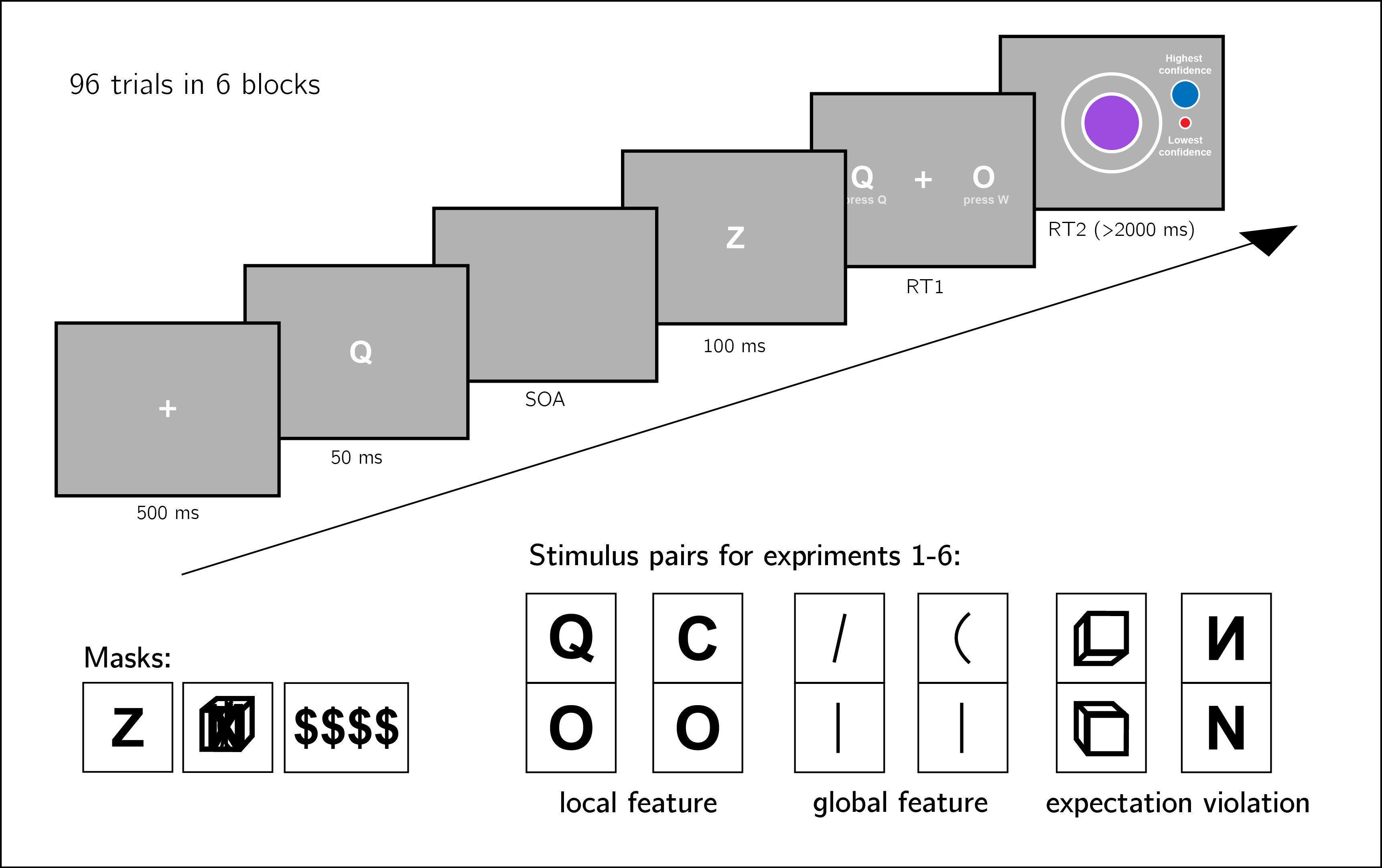
Figure 2.1: Experiment design. Metacognitive asymmetry effects were tested for six stimulus features in six separate experiments, encompassing three levels of abstraction: local features, global features, and expectation violations. The presented trial corresponds to the first stimulus pair, with Q and O as the two stimuli.
2.2.1 Randomization
The order and timing of experimental events was determined pseudo-randomly by the Mersenne Twister pseudorandom number generator, initialized in a way that ensures registration time-locking (Mazor, Mazor, and Mukamel 2019).
2.3 Data analysis
We used R (Version 3.6.0; R Core Team 2019) and the R-packages BayesFactor (Version 0.9.12.4.2; Morey and Rouder 2018), broom (Version 0.5.6; Robinson and Hayes 2020), cowplot (Version 1.0.0; Wilke 2019), dplyr (Version 1.0.4; Wickham et al. 2020), ggplot2 (Version 3.3.1; Wickham 2016), lmerTest (Version 3.1.2; Kuznetsova, Brockhoff, and Christensen 2017), lsr (Version 0.5; Navarro 2015), MESS (Version 0.5.6; Ekstrøm 2019), papaja (Version 0.1.0.9997; Aust and Barth 2020), pracma (Version 2.2.9; Borchers 2019), pwr (Version 1.3.0; Champely 2020), and tidyr (Version 1.1.0; Wickham and Henry 2020) for all our analyses.
For each of the six stimulus pairs [\(S_1\), \(S_2\)], we tested the following hypotheses:
- Hypothesis 1: Subjective confidence is higher for \(S_1\) responses than for \(S_2\) responses.
For each of the six stimulus pairs, we tested the null hypothesis that subjective confidence for \(S_1\) responses is equal to or lower than subjective confidence for the feature-absent stimulus (\(H_o: conf_{S_1}\leq Conf_{S_2}\)).
- Hypothesis 2: Metacognitive sensitivity, measured as the area under the response conditional ROC curves, is higher for \(S_1\) responses than for \(S_2\) responses.
For each of the six stimulus pairs, we tested the null hypothesis that metacognitive sensitivity for \(S_1\) responses is equal to or lower than metacognitive sensitivity for the \(S_2\) responses (\(H_o: auROC_{S_1}\leq auROC_{S_2}\)).
- Hypothesis 3: Metacognitive sensitivity, measured as the area under the response conditional ROC curves, is higher for \(S_1\) responses than for \(S_2\) responses, to a greater extent than expected from an equivalent equal-variance SDT model.
For each of the six stimulus pairs, we tested the null hypothesis that difference between metacognitive sensitivities for \(S_1\) and \(S_2\) responses is lower than the difference expected from an equivalent equal-variance SDT model (\(H_o: (auROC_{S_1}-auROC_{S_2})\leq (\widehat{auROC}_{S_1}-\widehat{auROC}_{S_2})\) where \(\widehat{auROC}\) is the expected auROC under an equal variance SDT model with equal sensitivity, criterion, and distribution of confidence ratings in incorrect responses).
- Hypothesis 4: \(S_1\) responses are faster on average than \(S_2\) responses.
For each of the six stimulus pairs, we tested the null hypothesis that log-transformed response times for \(S_1\) responses are equal to or higher than log-transformed response times for \(S_2\) responses (\(H_o: log(RT_{S_1})\geq log(RT_{S_2})\)).
Hypotheses 1 and 2 correspond to the effects of stimulus type on metacognitive bias and metacognitive sensitivity, respectively. Although these two measures are theoretically independent, both bias and sensitivity are found to vary between detection ‘yes’ and ‘no’ responses.
Based on pilot data and previous experiments examining near-threshold perceptual detection and discrimination, we did not expect a response bias (such that the probability of responding \(S_1\) is significantly different from 0.5 across participants). However, such a response bias, if found, may bias metacognitive asymmetry estimates as measured with response-conditional ROC curves. Hypothesis 3 was designed to confirm that metacognitive asymmetry is higher than that expected from an equivalent equal-variance SDT model with the same response bias, sensitivity, and distribution of confidence ratings in incorrect responses as in the actual data. We interpreted conflicting results for Hypotheses 2 and 3 as evidence for a metacognitive asymmetry that is driven or masked by a response bias.
Hypothesis 4 is motivated by two observations from previous studies. First, detection ‘yes’ responses are faster than detection ‘no’ responses (Mazor, Friston, and Fleming 2020). And second, when participants are not under strict time pressure, reaction time inversely scales with confidence (Henmon 1911; Calder-Travis et al. 2020; Pleskac and Busemeyer 2010; Moran, Teodorescu, and Usher 2015). Based on these findings, if \(S_1\) and \(S_2\) responses are similar to detection ‘yes’ and ‘no’ responses not only in explicit confidence judgments, but also in response times, we should also expect a response time difference for these stimulus pairs.
2.3.1 Dependent variables and analysis plan
Response conditional ROC curves were extracted by plotting the empirical cumulative distribution of confidence ratings for correct responses against the same cumulative distribution for incorrect responses. This was done separately for the two responses \(S_1\) and \(S_2\), resulting in two curves. The area under the response-conditional ROC curve is a measure of metacognitive sensitivity (Fleming and Lau 2014). The difference between the areas for the two responses is a measure of metacognitive asymmetry (Meuwese et al. 2014). This difference was used to test Hypothesis 2.
In order to test hypothesis 3, SDT-derived response-conditional ROC curves were plotted in the following way. For each response, we plotted the empirical cumulative distribution for incorrect responses on the x axis against the cumulative distribution for correct responses that would be expected in an equal-variance SDT model with matching sensitivity and response bias on the y axis. The difference between the areas of these theoretically derived response-conditional ROC curves was compared against the difference between the true response-conditional ROC curves.
For visualization purposes only, confidence ratings were divided into 20 bins, tailored for each participant to cover their dynamic range of confidence ratings.
For each of the six experiments, Hypotheses 1-4 were tested using a one tailed t-test at the group level with \(\alpha=0.05\). The summary statistic at the single subject level was difference in mean confidence between \(S_1\) and \(S_2\) responses for Hypothesis 1, difference in area under the response-conditional ROC curve between \(S_1\) and \(S_2\) responses (\(\Delta AUC\)) for Hypothesis 2, difference in \(\Delta AUC\) between true confidence distributions and SDT-derived confidence distributions for hypothesis 3, and difference in mean log response time between \(S_1\) and \(S_2\) responses for Hypothesis 4.
In addition, a Bayes factor was computed using the BayesFactor R package (Morey et al. 2015) and using a Jeffrey-Zellner-Siow (Cauchy) Prior with an rscale parameter of 0.65, representative of the similar standardized effect sizes we observe for Hypotheses 1-4 in our pilot data.
We based our inference on the resulting Bayes Factors.
2.3.2 Statistical power
Statistical power calculations were performed using the R-pwr packages pwr (Champely 2020) and PowerTOST (Labes et al. 2020).
Hypothesis 1 (MEAN CONFIDENCE): With 106 participants, we had statistical power of 95% to detect effects of size 0.32, which is less than the standardized effect size we observed for confidence in our pilot sample (\(d=0.66\)).
Hypothesis 2 (METACOGNITIVE ASYMMETRY): With 106 participants, we had statistical power of 95% to detect effects of size 0.32, which is less than the standardized effect size we observed for metacognitive sensitivity in our pilot sample (\(d=0.73\)).
Hypothesis 3 (METACOGNITIVE ASYMMETRY: CONTROL): With 106 participants, we had statistical power of 95% to detect effects of size 0.32, which is less than the standardized effect size we observed for metacognitive sensitivity, controlling for response bias, in our pilot sample (\(d=0.81\)).
Hypothesis 4 (RESPONSE TIME): With 106 participants, we had statistical power of 95% to detect effects of size 0.32, which is less than the standardized effect size we observed for response time in our pilot sample (\(d=0.61\)).
Finally, in case that the true effect size equals 0, a Bayes Factor with our chosen prior for the alternative hypothesis will support the null in 95 out of 100 repetitions, and will support the null with a \(BF_{01}\) higher than 3 in 79 out of 100 repetitions. In a case where the true effect size is sampled from a Cauchy distribution with a scale factor of 0.65, a Bayes Factor with our chosen prior for the alternative hypothesis will support the alternative hypothesis in 76 out of 100 repetitions, support the alternative hypothesis with a \(BF_{10}\) higher than 3 in 70 out of 100 repetitions, and support the null hypothesis with a \(BF_{01}\) higher than 3 in 15 out of 100 hypotheses (based on an adaptation of simulation code from Lakens 2016).
2.3.3 Rejection criteria
Participants were excluded for performing below 60% accuracy, for having extremely fast or slow reaction times (below 250 milliseconds or above 5 seconds in more than 25% of the trials), and for failing the comprehension check. Finally, for type-2 ROC curves to be generated, some responses must be incorrect, and for them to be informative some variability in confidence ratings is necessary. Thus, participants who committed less than two of each error type (for example, mistaking a Q of O and mistaking an O for Q), or who reported less than two different confidence levels for each of the two responses were excluded from all analyses.
Trials with response time below 250 milliseconds or above 5 seconds were excluded.
2.4 Data availability
All raw data is fully available on OSF and on the study’s GitHub respository: https://github.com/matanmazor/asymmetry.
2.5 Code availability
All analysis code is openly shared on the study’s GitHub repository: https://github.com/matanmazor/asymmetry. For complete reproducibility, the RMarkdown file used to generate the final version of the manuscript, including the generation of all figures and extraction of all test statistics, is also available on our GitHub repository.
2.6 Deviations from pre-registration
Stimulus used for backward masking: We planned to use the same stimulus (the letter Z) for backward masking in all six experiments. This mask was effective in Experiments 1 and 2, but in Experiment 3 overly high accuracy levels indicated that for these stimuli the mask was not salient enough. For a subset of participants in Exp. 3, an overlay of all 7 stimuli from experiments 3-6 (vertical, tilted, and curved lines, upward-tilted and downward-tilted cubes, and normal and flipped Ns) was used. For the remaining participants and experiments, we used four dollar signs as our mask. See Fig. 2.1 for depictions of the three masks.
Rejection criteria: In our pre-registration we explain that informative response-conditional ROC curves can only be generated if participants make errors. When analyzing the data we came to realize that an additional prerequisite for response-conditional ROC curves to be informative is that the variance in confidence ratings is higher than zero, otherwise the curve is diagonal. We therefore required that participants report at least two different confidence levels for each response. Participants that did not meet this additional criterion were excluded from all analyses.
Monetary compensation: For some of the experiments, we noticed that participants completed the experiment more quickly than what we had originally estimated. We therefore reduced our offered payment for some of the experiments, while maintaining a median hourly wage of £6 or higher.